A query can read fewer columns and partitions yet remain slow because a join multiplies rows or one task receives most of a shuffle. Read the plan from the scan toward the output, then compare it with runtime evidence. SQL text alone does not establish the amount of work.
Follow one analytical query
Assume a Delta-aware Spark session and an events table with columns event_date, device_id, tenant_id and kwh. A device dimension has one current row per device.
EXPLAIN FORMATTED
SELECT e.tenant_id, SUM(e.kwh) AS energy_kwh
FROM analytics.events e
JOIN analytics.devices d
  ON e.device_id = d.device_id
WHERE e.event_date >= DATE '2026-10-01'
  AND e.event_date < DATE '2026-10-08'
  AND d.status = 'active'
GROUP BY e.tenant_id;
The explanation below is an operator checklist, not captured output from a particular Spark release. Data-source versions and adaptive planning change the rendered plan.
| Plan evidence | Question it can answer | What it cannot prove alone |
|---|---|---|
| PartitionFilters or equivalent scan metadata | Did an eligible partition predicate reach the scan? | Exactly how many physical bytes were avoided |
| PushedFilters or data-source predicates | Did filtering move into the reader? | Every matching row group or file could be skipped |
| ReadSchema or projected columns | Which columns does the scan require? | Total object traffic, metadata reads or cache effects |
| BroadcastHashJoin | Is one join side broadcast to workers? | The build input safely fits memory under real concurrency |
| Exchange followed by aggregation/sort | Where are rows redistributed? | Whether the shuffle is balanced |
| Adaptive final plan | What plan ran after runtime adjustments? | The same plan will be chosen for another input distribution |
First inspect both scan inputs. A selective dimension predicate may reduce the dimension but leave the fact scan large. Dynamic pruning can help in supported cases; its presence must be verified in the selected engine and executed plan.
Then check the join’s row counts. If a device appears twice in the dimension, its events can contribute twice to the sum. An otherwise efficient physical plan cannot repair that modelling error.
Runtime work separates diagnoses
Collect the table version, SQL, parameters, engine settings and cache state for a baseline run. Compare files or partitions read, input bytes and rows, output rows, shuffle read/write, spill, task-duration distribution and elapsed time.
| Observation | Plausible cause | Focused experiment |
|---|---|---|
| Most files read for a narrow date query | Missing eligible filter, wrong partition field or unhelpful statistics | Confirm table layout and inspect scan predicates |
| Few input bytes, huge join output | Non-unique join keys or intended many-to-many expansion | Count matches per business key before changing resources |
| Similar bytes, much slower elapsed time | Queueing, contention, remote latency or changed parallelism | Compare wait time and stage timing with a known-good run |
| One task is much slower than peers | Hot key, uneven file split or expensive records | Inspect per-task input and key distribution |
| Heavy spill during a join or sort | Working state exceeds available execution memory | Reduce unnecessary rows/width and test partition or join strategy |
| Long planning delay before tasks start | File discovery, metadata or catalog overhead | Compare file count and planning time after supported maintenance |
Spill writes intermediate working data to disk when it cannot stay in the allotted memory. Some spill is a supported execution strategy; repeated large spill can dominate latency. More memory per worker may reduce spill but can also reduce affordable parallelism.
SQL shape can hide a useful filter
A direct half-open date range makes intended coverage clear. A function or cast can sometimes be rewritten by the optimizer; it does not universally disable pruning. Inspect the emitted plan for the actual expression and connector.
Native expressions give optimizers more visibility than opaque Python user-defined functions (UDFs). A UDF can prevent useful rewrites or add serialization cost. Use one when its behavior is required and measure the resulting plan.
Likewise, LIMIT bounds returned rows; a grouped query may still scan and aggregate all eligible input before returning those rows.
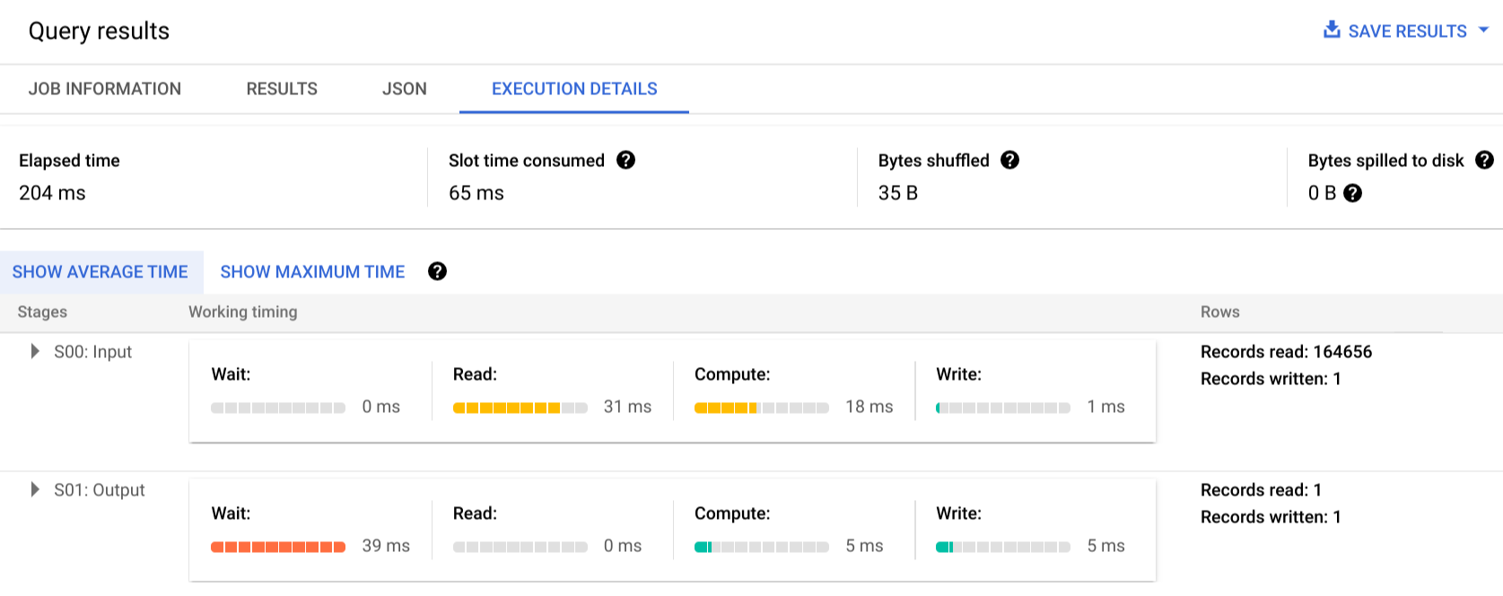
Inspect wait, read, compute and write time alongside records read and written for each stage. The screenshot illustrates the evidence available; timings belong to that example job.
Plans belong to their engine
Spark SQL and DataFrame APIs can produce equivalent optimized plans. Resilient Distributed Dataset (RDD) code gives more manual control and generally exposes less relational structure to the SQL optimizer. See Spark plans, repartitioning and adaptive query execution for execution partitions and skew remedies.
DuckDB’s EXPLAIN ANALYZE executes the query and reports operator timing and cardinality. PostgreSQL’s EXPLAIN workflow adds buffer and access-path reasoning. BigQuery exposes distributed execution stages and job metadata; the worked investigation uses those signals.
Compare one change at a time against the same input and result contract. Physical-layout experiments belong with partitioning and file sizing; adding compute before locating the expensive operator can preserve the same bottleneck at higher cost.